ordpy: A Python Package for Data Analysis with Permutation Entropy and Ordinal Network Methods
ordpy is a pure Python module 1 that implements data analysis methods based
on Bandt and Pompe’s 2 symbolic encoding scheme.
Note
If you have used ordpy in a scientific publication, we would appreciate
citations to the following reference 1:
A. A. B. Pessa, H. V. Ribeiro, ordpy: A Python package for data analysis with permutation entropy and ordinal network methods, Chaos 31, 063110 (2021). arXiv:2102.06786
@misc{pessa2021ordpy,
  title         = {ordpy: A Python package for data analysis with permutation entropy and ordinal network methods},
  author        = {Arthur A. B. Pessa and Haroldo V. Ribeiro},
  journal       = {Chaos: An Interdisciplinary Journal of Nonlinear Science},
  volume        = {31},
  number        = {6},
  pages         = {063110},
  year          = {2021},
  doi           = {10.1063/5.0049901},
 }
ordpy implements the following data analysis methods:
Released on version 1.0.0 (February 2021):
Multiscale complexity-entropy plane for time series 6 and images 7;
Tsallis 8 and Rényi 9 generalized complexity-entropy curves for time series and images;
Global node entropy of ordinal networks for time series 13, 11 and images 12.
Missing ordinal patterns 14 and missing transitions between ordinal patterns 11 for time series and images.
Released on version 1.1.0 (January 2023):
Weighted permutation entropy for time series 15 and images;
Fisher-Shannon plane for time series 16 and images;
Permutation Jensen-Shannon distance for time series 17 and images;
Four pattern permutation contrasts (up-down balance, persistence, rotational-asymmetry, and up-down scaling.) for time series 18;
Smoothness-structure plane for images 19.
Released on version 1.2.0 (April 2025):
Two-by-two ordinal patterns for images 21.
References
- 1(1,2,3)
Pessa, A. A., & Ribeiro, H. V. (2021). ordpy: A Python package for data analysis with permutation entropy and ordinal networks methods. Chaos, 31, 063110.
- 2(1,2,3,4,5,6,7)
Bandt, C., & Pompe, B. (2002). Permutation entropy: A Natural Complexity Measure for Time Series. Physical Review Letters, 88, 174102.
- 3(1,2,3)
Ribeiro, H. V., Zunino, L., Lenzi, E. K., Santoro, P. A., & Mendes, R. S. (2012). Complexity-Entropy Causality Plane as a Complexity Measure for Two-Dimensional Patterns. PLOS ONE, 7, e40689.
- 4(1,2)
Lopez-Ruiz, R., Mancini, H. L., & Calbet, X. (1995). A Statistical Measure of Complexity. Physics Letters A, 209, 321-326.
- 5(1,2)
Rosso, O. A., Larrondo, H. A., Martin, M. T., Plastino, A., & Fuentes, M. A. (2007). Distinguishing Noise from Chaos. Physical Review Letters, 99, 154102.
- 6
Zunino, L., Soriano, M. C., & Rosso, O. A. (2012). Distinguishing Chaotic and Stochastic Dynamics from Time Series by Using a Multiscale Symbolic Approach. Physical Review E, 86, 046210.
- 7
Zunino, L., & Ribeiro, H. V. (2016). Discriminating Image Textures with the Multiscale Two-Dimensional Complexity-Entropy Causality Plane. Chaos, Solitons & Fractals, 91, 679-688.
- 8(1,2,3)
Ribeiro, H. V., Jauregui, M., Zunino, L., & Lenzi, E. K. (2017). Characterizing Time Series Via Complexity-Entropy Curves. Physical Review E, 95, 062106.
- 9(1,2,3)
Jauregui, M., Zunino, L., Lenzi, E. K., Mendes, R. S., & Ribeiro, H. V. (2018). Characterization of Time Series via Rényi Complexity-Entropy Curves. Physica A, 498, 74-85.
- 10(1,2)
Small, M. (2013). Complex Networks From Time Series: Capturing Dynamics. In 2013 IEEE International Symposium on Circuits and Systems (ISCAS2013) (pp. 2509-2512). IEEE.
- 11(1,2,3,4,5,6,7)
Pessa, A. A., & Ribeiro, H. V. (2019). Characterizing Stochastic Time Series With Ordinal Networks. Physical Review E, 100, 042304.
- 12(1,2,3,4)
Pessa, A. A., & Ribeiro, H. V. (2020). Mapping Images Into Ordinal Networks. Physical Review E, 102, 052312.
- 13(1,2)
McCullough, M., Small, M., Iu, H. H. C., & Stemler, T. (2017). Multiscale Ordinal Network Analysis of Human Cardiac Dynamics. Philosophical Transactions of the Royal Society A, 375, 20160292.
- 14(1,2)
Amigó, J. M., Zambrano, S., & Sanjuán, M. A. F. (2007). True and False Forbidden Patterns in Deterministic and Random Dynamics. Europhysics Letters, 79, 50001.
- 15(1,2)
Fadlallah B., Chen, B., Keil A. & Príncipe, J. (2013). Weighted-permutation entropy: a complexity measure for time series incorporating amplitude information. Physical Review E, 97, 022911.
- 16(1,2)
Olivares, F., Plastino, A., & Rosso, O. A. (2012). Contrasting chaos with noise via local versus global information quantifiers. Physics Letters A, 376, 1577–1583.
- 17(1,2)
Zunino L., Olivares, F., Ribeiro H. V. & Rosso, O. A. (2022). Permutation Jensen-Shannon distance: A versatile and fast symbolic tool for complex time-series analysis. Physical Review E, 105, 045310.
- 18(1,2)
Bandt, C. (2023). Statistics and contrasts of order patterns in univariate time series, Chaos, 33, 033124.
- 19(1,2,3,4)
Bandt, C., & Wittfeld, K. (2023). Two new parameters for the ordinal analysis of images, Chaos, 33, 043124.
- 20(1,2)
Martin, M. T., Plastino, A., & Rosso, O. A. (2006). Generalized Statistical Complexity Measures: Geometrical and Analytical Properties, Physica A, 369, 439–462.
- 21(1,2,3)
Tarozo, M. M., Pessa, A. A., Zunino, L., Rosso, O. A., Perc, M. & Ribeiro, H. V. (2025). Two-by-two ordinal patterns in art paintings. PNAS Nexus, 4, pgaf092.
Installing
Ordpy can be installed via the command line using
pip install ordpy
or you can directly clone its git repository:
git clone https://github.com/arthurpessa/ordpy.git
cd ordpy
pip install -e .
Basic usage
We provide a notebook
illustrating how to use ordpy. This notebook reproduces all figures of our
article 1. The code below shows simple applications of ordpy.
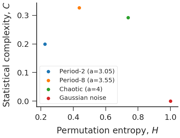
#Complexity-entropy plane for logistic map and Gaussian noise.

import numpy as np
import ordpy
from matplotlib import pylab as plt

def logistic(a=4, n=100000, x0=0.4):
    x = np.zeros(n)
    x[0] = x0
    for i in range(n-1):
        x[i+1] = a*x[i]*(1-x[i])
    return(x)

time_series = [logistic(a) for a in [3.05, 3.55, 4]]
time_series += [np.random.normal(size=100000)]

HC = [ordpy.complexity_entropy(series, dx=4) for series in time_series]


f, ax = plt.subplots(figsize=(8.19, 6.3))

for HC_, label_ in zip(HC, ['Period-2 (a=3.05)',
                            'Period-8 (a=3.55)',
                            'Chaotic (a=4)',
                            'Gaussian noise']):
    ax.scatter(*HC_, label=label_, s=100)

ax.set_xlabel('Permutation entropy, $H$')
ax.set_ylabel('Statistical complexity, $C$')

ax.legend()
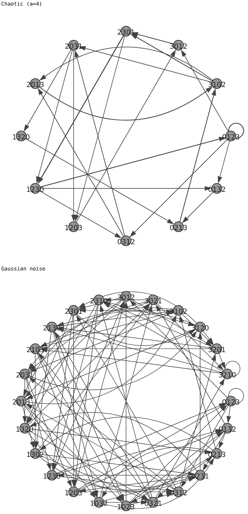
#Ordinal networks for logistic map and Gaussian noise.

import numpy as np
import igraph
import ordpy
from matplotlib import pylab as plt
from IPython.core.display import display, SVG

def logistic(a=4, n=100000, x0=0.4):
    x = np.zeros(n)
    x[0] = x0
    for i in range(n-1):
        x[i+1] = a*x[i]*(1-x[i])
    return(x)

time_series = [logistic(a=4), np.random.normal(size=100000)]

vertex_list, edge_list, edge_weight_list = list(), list(), list()
for series in time_series:
    v_, e_, w_   = ordpy.ordinal_network(series, dx=4)
    vertex_list += [v_]
    edge_list   += [e_]
    edge_weight_list += [w_]

def create_ig_graph(vertex_list, edge_list, edge_weight):

    G = igraph.Graph(directed=True)

    for v_ in vertex_list:
        G.add_vertex(v_)

    for [in_, out_], weight_ in zip(edge_list, edge_weight):
        G.add_edge(in_, out_, weight=weight_)

    return G

graphs = []

for v_, e_, w_ in zip(vertex_list, edge_list, edge_weight_list):
    graphs += [create_ig_graph(v_, e_, w_)]

def igplot(g):
    f = igraph.plot(g,
                    layout=g.layout_circle(),
                    bbox=(500,500),
                    margin=(40, 40, 40, 40),
                    vertex_label = [s.replace('|','') for s in g.vs['name']],
                    vertex_label_color='#202020',
                    vertex_color='#969696',
                    vertex_size=20,
                    vertex_font_size=6,
                    edge_width=(1 + 8*np.asarray(g.es['weight'])).tolist(),
                   )
    return f

for graph_, label_ in zip(graphs, ['Chaotic (a=4)',
                                   'Gaussian noise']):
    print(label_)
    display(SVG(igplot(graph_)._repr_svg_()))
List of functions
- ordpy.complexity_entropy(data, dx=3, dy=1, taux=1, tauy=1, probs=False, tie_precision=None)[source]
Calculates permutation entropy2 and statistical complexity4,5 using an ordinal distribution obtained from data.
- Parameters
data (array) – Array object in the format \([x_{1}, x_{2}, x_{3}, \ldots ,x_{n}]\) or \([[x_{11}, x_{12}, x_{13}, \ldots, x_{1m}], \ldots, [x_{n1}, x_{n2}, x_{n3}, \ldots, x_{nm}]]\) or an ordinal probability distribution (such as the ones returned by
ordpy.ordinal_distribution()).dx (int) – Embedding dimension (horizontal axis) (default: 3).
dy (int) – Embedding dimension (vertical axis); it must be 1 for time series (default: 1).
taux (int) – Embedding delay (horizontal axis) (default: 1).
tauy (int) – Embedding delay (vertical axis) (default: 1).
probs (boolean) – If True, it assumes data is an ordinal probability distribution. If False, data is expected to be a one- or two-dimensional array (default: False).
tie_precision (None, int) – If not None, data is rounded with tie_precision decimal numbers (default: None).
- Returns
Values of normalized permutation entropy and statistical complexity.
- Return type
tuple
Examples
>>> complexity_entropy([4,7,9,10,6,11,3], dx=2)
(0.9182958340544894, 0.06112816548804511)
>>>
>>> p = ordinal_distribution([4,7,9,10,6,11,3], dx=2, return_missing=True)[1]
>>> complexity_entropy(p, dx=2, probs=True)
(0.9182958340544894, 0.06112816548804511)
>>>
>>> complexity_entropy([[1,2,1],[8,3,4],[6,7,5]], dx=2, dy=2)
(0.3271564379782973, 0.2701200547320647)
>>>
>>> complexity_entropy([1/3, 1/15, 4/15, 2/15, 1/5, 0], dx=3, probs=True)
(0.8314454838586238, 0.16576716623440763)
>>>
>>> complexity_entropy([[1,2,1,4],[8,3,4,5],[6,7,5,6]],dx=3, dy=2)
(0.21070701155008006, 0.20704765093242872)
- ordpy.fisher_shannon(data, dx=3, dy=1, taux=1, tauy=1, probs=False, tie_precision=None)[source]
Calculates permutation entropy2 and Fisher information16 using an ordinal distribution obtained from data.
- Parameters
data (array) – Array object in the format \([x_{1}, x_{2}, x_{3}, \ldots ,x_{n}]\) or \([[x_{11}, x_{12}, x_{13}, \ldots, x_{1m}], \ldots, [x_{n1}, x_{n2}, x_{n3}, \ldots, x_{nm}]]\) or an ordinal probability distribution (such as the ones returned by
ordpy.ordinal_distribution()).dx (int) – Embedding dimension (horizontal axis) (default: 3).
dy (int) – Embedding dimension (vertical axis); it must be 1 for time series (default: 1).
taux (int) – Embedding delay (horizontal axis) (default: 1).
tauy (int) – Embedding delay (vertical axis) (default: 1).
probs (boolean) – If True, it assumes data is an ordinal probability distribution. If False, data is expected to be a one- or two-dimensional array (default: False).
tie_precision (None, int) – If not None, data is rounded with tie_precision decimal numbers (default: None).
- Returns
Values of normalized permutation entropy and Fisher information.
- Return type
tuple
Examples
>>> fisher_shannon([4,7,9,10,6,11,3], dx=2)
(0.9182958340544896, 0.028595479208968325)
>>>
>>> p = ordinal_distribution([4,7,9,10,6,11,3], dx=2, return_missing=True)[1]
>>> fisher_shannon(p, dx=2, probs=True)
(0.9182958340544896, 0.028595479208968325)
>>>
>>> fisher_shannon([[1,2,1],[8,3,4],[6,7,5]], dx=2, dy=2)
(0.32715643797829735, 1.0)
>>>
>>> fisher_shannon([1/3, 1/15, 2/15, 3/15, 4/15, 0], dx=3, probs=True)
(0.8314454838586239, 0.19574180681374548)
>>>
>>> fisher_shannon([[1,2,1,4],[8,3,4,5],[6,7,5,6]], dx=3, dy=2)
(0.2107070115500801, 1.0)
- ordpy.global_node_entropy(data, dx=3, dy=1, taux=1, tauy=1, overlapping=True, connections='all', tie_precision=None)[source]
Calculates global node entropy11,13 for an ordinal network obtained from data. (Assumes directed and weighted edges).
- Parameters
data (array, return of
ordpy.ordinal_network()) – Array object in the format \([x_{1}, x_{2}, x_{3}, \ldots ,x_{n}]\) or \([[x_{11}, x_{12}, x_{13}, \ldots, x_{1m}], \ldots, [x_{n1}, x_{n2}, x_{n3}, \ldots, x_{nm}]]\) or an ordinal network returned byordpy.ordinal_network()*.dx (int) – Embedding dimension (horizontal axis) (default: 3).
dy (int) – Embedding dimension (vertical axis); it must be 1 for time series (default: 1).
taux (int) – Embedding delay (horizontal axis) (default: 1).
tauy (int) – Embedding delay (vertical axis) (default: 1).
overlapping (boolean) – If True, data is partitioned into overlapping sliding windows (default: True). If False, adjacent partitions are non-overlapping.
connections (str) – The ordinal network is constructed using ‘all’ permutation successions in a symbolic sequence or only ‘horizontal’ or ‘vertical’ successions. Parameter only valid for image data (default: ‘all’).
tie_precision (None, int) – If not None, data is rounded with tie_precision decimal numbers (default: None).
- Returns
Value of global node entropy.
- Return type
float
Notes
- *
In case data is an ordinal network returned by
ordpy.ordinal_network(), the parameters ofordpy.global_node_entropy()are inferred from the network.
Examples
>>> global_node_entropy([1,2,3,4,5,6,7,8,9], dx=2)
0.0
>>>
>>> global_node_entropy(ordinal_network([1,2,3,4,5,6,7,8,9], dx=2))
0.0
>>>
>>> global_node_entropy(np.random.uniform(size=100000), dx=3)
1.4988332319747597
>>>
>>> global_node_entropy(random_ordinal_network(dx=3))
1.5
>>>
>>> global_node_entropy([[1,2,1,4],[8,3,4,5],[6,7,5,6]], dx=2, dy=2, connections='horizontal')
0.25
>>>
>>> global_node_entropy([[1,2,1,4],[8,3,4,5],[6,7,5,6]], dx=2, dy=2, connections='vertical')
0.0
- ordpy.logq(x, q=1)[source]
Calculates the q-logarithm of x.
- Parameters
x (float, array) – Real number or array containing real numbers.
q (float) – Tsallis’s q parameter (default: 1).
- Returns
Value or array of values containing the q-logarithm of x.
- Return type
float or array
Notes
The q-logarithm of x is defined as†
\[\]log_q (x) = frac{x^{1-q} - 1}{1-q}~~text{for}~~qneq 1
and \(\log_q (x) = \log (x)\) for \(q=1\).
- †
Tsallis, C. (2009). Introduction to Nonextensive Statistical Mechanics: Approaching a Complex World. Springer.
Examples
>>> logq(np.math.e)
1.0
>>>
>>> logq([np.math.e for i in range(5)])
array([1., 1., 1., 1., 1.])
- ordpy.maximum_complexity_entropy(dx=3, dy=1, m=1)[source]
Generates data corresponding to values of normalized permutation entropy and statistical complexity which delimit the upper boundary in the complexity-entropy causality plane20,‡.
- Parameters
dx (int) – Embedding dimension (horizontal axis) (default: 3).
dy (int) – Embedding dimension (vertical axis); must be 1 for time series (default: 1).
m (int) – The length of the returned array containing values of permutation entropy and statistical complexity is given by \([(d_x \times d_y)!-1] \times m\).
- Returns
Values of normalized permutation entropy and statistical complexity belonging to the upper limiting curve of the complexity-entropy causality plane.
- Return type
array
Notes
- ‡
This function was adapted from Sebastian Sippel et al., statcomp: Statistical Complexity and Information Measures for Time Series Analysis, version 0.1.0. (Computer Software in R).
Examples
>>> maximum_complexity_entropy(dx=3, dy=1, m=1)
array([[-0.        , -0.        ],
       [ 0.38685281,  0.27123863],
       [ 0.61314719,  0.29145164],
       [ 0.77370561,  0.22551573],
       [ 0.8982444 ,  0.12181148]])
>>>
>>> maximum_complexity_entropy(dx=3, dy=1, m=2)
array([[-0.        , -0.        ],
       [ 0.251463  ,  0.19519391],
       [ 0.38685281,  0.27123863],
       [ 0.57384034,  0.28903864],
       [ 0.61314719,  0.29145164],
       [ 0.76241899,  0.2294088 ],
       [ 0.77370561,  0.22551573],
       [ 0.89621768,  0.12320718],
       [ 0.8982444 ,  0.12181148],
       [ 1.        ,  0.        ]])
- ordpy.minimum_complexity_entropy(dx=3, dy=1, size=100)[source]
Generates data corresponding to values of normalized permutation entropy and statistical complexity which delimit the lower boundary in the complexity-entropy causality plane20,§.
- Parameters
dx (int) – Embedding dimension (horizontal axis) (default: 3).
dy (int) – Embedding dimension (vertical axis); must be 1 for time series (default: 1).
size (int) – The length of the array returned containing pairs of values of permutation entropy and statistical complexity.
- Returns
Values of normalized permutation entropy and statistical complexity belonging to the lower limiting curve of the complexity-entropy causality plane.
- Return type
array
Notes
- §
This function was adapted from Sebastian Sippel et al., statcomp: Statistical Complexity and Information Measures for Time Series Analysis, version 0.1.0. (Computer Software in R).
Examples
>>> minimum_complexity_entropy(dx=3, size=10)
array([[-0.        , -0.        ],
       [ 0.25534537,  0.17487933],
       [ 0.43376898,  0.21798915],
       [ 0.57926767,  0.21217508],
       [ 0.70056313,  0.18118876],
       [ 0.80117413,  0.1378572 ],
       [ 0.88242522,  0.09085847],
       [ 0.94417789,  0.04723328],
       [ 0.98476216,  0.01396083],
       [ 1.        ,  0.        ]])
>>>
>>> minimum_complexity_entropy(dx=4, size=5)
array([[-0.00000000e+00, -0.00000000e+00],
       [ 4.09625322e-01,  2.10690777e-01],
       [ 6.90580872e-01,  1.84011590e-01],
       [ 8.96072453e-01,  8.64190054e-02],
       [ 1.00000000e+00, -3.66606083e-16]])
- ordpy.missing_links(data, dx=3, dy=1, return_fraction=True, return_missing=True, tie_precision=None)[source]
Identifies transitions between ordinal patterns (permutations) not occurring in data. (These transtitions correspond to directed edges in ordinal networks11.) Assumes overlapping windows and unitary embedding delay. In case dx>1 and dy>1, both ‘horizontal’ and ‘vertical’ connections are considered (see
ordpy.ordinal_network()).- Parameters
data (array, return of
ordpy.ordinal_network()) – Array object in the format \([x_{1}, x_{2}, x_{3}, \ldots ,x_{n}]\) or \([[x_{11}, x_{12}, x_{13}, \ldots, x_{1m}], \ldots, [x_{n1}, x_{n2}, x_{n3}, \ldots, x_{nm}]]\) or the nodes, edges and edge weights returned byordpy.ordinal_network().dx (int) – Embedding dimension (horizontal axis) (default: 3)
dy (int) – Embedding dimension (vertical axis); must be 1 for time series (default: 1).
return_fraction (boolean) – if True, returns the fraction of missing links among ordinal patterns relative to the total number of possible links (transitions) for given values of dx and dy (default: True). If False, returns the raw number of missing links.
return_missing (boolean) – if True, returns the missing links in data; if False, it only returns the fraction/number of these missing links.
tie_precision (None, int) – If not None, data is rounded with tie_precision decimal numbers (default: None).
- Returns
Tuple containing an array and a float indicating missing links and their relative fraction (or raw number).
- Return type
tuple
Examples
>>> missing_links([4,7,9,10,6,11,3], dx=2, return_fraction=False)
(array([['1|0', '1|0']], dtype='<U3'), 1)
>>>
>>> missing_links(ordinal_network([4,7,9,10,6,11,3], dx=2), dx=2, return_fraction=True)
(array([['1|0', '1|0']], dtype='<U3'), 0.25)
>>>
>>> missing_links([4,7,9,10,6,11,3,5,6,2,3,1], dx=3, return_fraction=False)
(array([['0|1|2', '0|2|1'],
        ['0|2|1', '1|0|2'],
        ['0|2|1', '1|2|0'],
        ['0|2|1', '2|1|0'],
        ['1|0|2', '0|1|2'],
        ['1|0|2', '0|2|1'],
        ['1|2|0', '0|2|1'],
        ['2|0|1', '2|1|0'],
        ['2|1|0', '1|0|2'],
        ['2|1|0', '1|2|0'],
        ['2|1|0', '2|1|0']], dtype='<U5'), 11)
- ordpy.missing_patterns(data, dx=3, dy=1, taux=1, tauy=1, return_fraction=True, return_missing=True, probs=False, tie_precision=None)[source]
Identifies ordinal patterns (permutations) not occurring in data14.
- Parameters
data (array, return of
ordpy.ordinal_distribution()) – Array object in the format \([x_{1}, x_{2}, x_{3}, \ldots ,x_{n}]\) or \([[x_{11}, x_{12}, x_{13}, \ldots, x_{1m}], \ldots, [x_{n1}, x_{n2}, x_{n3}, \ldots, x_{nm}]]\) or the ordinal patterns and probabilities returned byordpy.ordinal_distribution()with return_missing=True.dx (int) – Embedding dimension (horizontal axis) (default: 3).
dy (int) – Embedding dimension (vertical axis); must be 1 for time series (default: 1).
taux (int) – Embedding delay (horizontal axis) (default: 1).
tauy (int) – Embedding delay (vertical axis) (default: 1).
return_fraction (boolean) – if True, returns the fraction of missing ordinal patterns relative to the total number of ordinal patterns for given values of dx and dy (default: True); if False, returns the raw number of missing patterns.
return_missing (boolean) – if True, returns the missing ordinal patterns in data (default: True); if False, it only returns the fraction/number of these missing patterns.
probs (boolean) – If True, assumes data to be the return of
ordpy.ordinal_distribution()with return_missing=True. If False, data is expected to be a one- or two-dimensional array (default: False).tie_precision (None, int) – If not None, data is rounded with tie_precision decimal numbers (default: None).
- Returns
Tuple containing an array and a float indicating missing ordinal patterns and their relative fraction (or raw number).
- Return type
tuple
Examples
>>> missing_patterns([4,7,9,10,6,11,3], dx=2, return_fraction=False)
(array([], shape=(0, 2), dtype=int64), 0)
>>>
>>> missing_patterns([4,7,9,10,6,11,3,5,6,2,3,1], dx=3, return_fraction=True, return_missing=False)
0.3333333333333333
>>>
>>> missing_patterns(ordinal_distribution([4,7,9,10,6,11,3], dx=2, return_missing=True), dx=2, probs=True)
(array([], shape=(0, 2), dtype=int64), 0.0)
>>>
>>> missing_patterns(ordinal_distribution([4,7,9,10,6,11,3], dx=3, return_missing=True), dx=3, probs=True)
(array([[0, 2, 1],
        [1, 2, 0],
        [2, 1, 0]]), 0.5)
- ordpy.ordinal_distribution(data, dx=3, dy=1, taux=1, tauy=1, return_missing=False, tie_precision=None, ordered=False)[source]
Applies the Bandt and Pompe2 symbolization approach to obtain a probability distribution of ordinal patterns (permutations) from data.
- Parameters
data (array) – Array object in the format \([x_{1}, x_{2}, x_{3}, \ldots ,x_{n}]\) or \([[x_{11}, x_{12}, x_{13}, \ldots, x_{1m}], \ldots, [x_{n1}, x_{n2}, x_{n3}, \ldots, x_{nm}]]\).
dx (int) – Embedding dimension (horizontal axis) (default: 3).
dy (int) – Embedding dimension (vertical axis); it must be 1 for time series (default: 1).
taux (int) – Embedding delay (horizontal axis) (default: 1).
tauy (int) – Embedding delay (vertical axis) (default: 1).
return_missing (boolean) – If True, it returns ordinal patterns not appearing in the symbolic sequence obtained from data. If False, these missing patterns (permutations) are omitted (default: False).
tie_precision (None, int) – If not None, data is rounded with tie_precision decimal numbers (default: None).
ordered (boolean) – If True, it also returns ordinal patterns not appearing in the symbolic sequence obtained from data in ascending ordered. The return_missing parameter must also be True.
- Returns
Tuple containing two arrays, one with the ordinal patterns and another with their corresponding probabilities.
- Return type
tuple
Examples
>>> ordinal_distribution([4,7,9,10,6,11,3], dx=2)
(array([[0, 1],
        [1, 0]]),
 array([0.66666667, 0.33333333]))
>>>
>>> ordinal_distribution([4,7,9,10,6,11,3], dx=3, return_missing=True)
(array([[0, 1, 2],
        [1, 0, 2],
        [2, 0, 1],
        [0, 2, 1],
        [1, 2, 0],
        [2, 1, 0]]),
 array([0.4, 0.2, 0.4, 0. , 0. , 0. ]))
>>>
>>> ordinal_distribution([[1,2,1],[8,3,4],[6,7,5]], dx=2, dy=2)
(array([[0, 1, 3, 2],
        [1, 0, 2, 3],
        [1, 2, 3, 0]]),
 array([0.5 , 0.25, 0.25]))
>>>
>>> ordinal_distribution([[1,2,1,4],[8,3,4,5],[6,7,5,6]], dx=2, dy=2, taux=2)
(array([[0, 1, 3, 2],
        [0, 2, 1, 3],
        [1, 3, 2, 0]]),
 array([0.5 , 0.25, 0.25]))
- ordpy.ordinal_network(data, dx=3, dy=1, taux=1, tauy=1, normalized=True, overlapping=True, directed=True, connections='all', tie_precision=None)[source]
Maps a data set into the elements (nodes, edges and edge weights) of its corresponding ordinal network representation10,11,12.
- Parameters
data (array) – Array object in the format \([x_{1}, x_{2}, x_{3}, \ldots ,x_{n}]\) or \([[x_{11}, x_{12}, x_{13}, \ldots, x_{1m}], \ldots, [x_{n1}, x_{n2}, x_{n3}, \ldots, x_{nm}]]\).
dx (int) – Embedding dimension (horizontal axis) (default: 3).
dy (int) – Embedding dimension (vertical axis); it must be 1 for time series (default: 1).
taux (int) – Embedding delay (horizontal axis) (default: 1).
tauy (int) – Embedding delay (vertical axis) (default: 1).
normalized (boolean) – If True, edge weights represent transition probabilities between permutations (default: True). If False, edge weights are transition counts.
overlapping (boolean) – If True, data is partitioned into overlapping sliding windows (default: True). If False, adjacent partitions are non-overlapping.
directed (boolean) – If True, ordinal network edges are directed (default: True). If False, edges are undirected.
connections (str) – The ordinal network is constructed using ‘all’ permutation successions in a symbolic sequence or only ‘horizontal’ or ‘vertical’ successions. Parameter only valid for image data (default: ‘all’).
tie_precision (None, int) – If not None, data is rounded with tie_precision decimal numbers (default: None).
- Returns
Tuple containing three arrays corresponding to nodes, edges and edge weights of an ordinal network.
- Return type
tuple
Examples
>>> ordinal_network([4,7,9,10,6,11,8,3,7], dx=2, normalized=False)
(array(['0|1', '1|0'], dtype='<U3'),
 array([['0|1', '0|1'],
        ['0|1', '1|0'],
        ['1|0', '0|1'],
        ['1|0', '1|0']], dtype='<U3'),
 array([2, 2, 2, 1]))
>>>
>>> ordinal_network([4,7,9,10,6,11,8,3,7], dx=2, overlapping=False, normalized=False)
(array(['0|1', '1|0'], dtype='<U3'),
 array([['0|1', '0|1'],
        ['0|1', '1|0']], dtype='<U3'),
 array([2, 1]))
>>>
>>> ordinal_network([[1,2,1],[8,3,4],[6,7,5]], dx=2, dy=2, normalized=False)
(array(['0|1|3|2', '1|0|2|3', '1|2|3|0'], dtype='<U7'),
 array([['0|1|3|2', '1|0|2|3'],
        ['0|1|3|2', '1|2|3|0'],
        ['1|0|2|3', '0|1|3|2'],
        ['1|2|3|0', '0|1|3|2']], dtype='<U7'),
 array([1, 1, 1, 1]))
>>>
>>> ordinal_network([[1,2,1],[8,3,4],[6,7,5]], dx=2, dy=2, normalized=True, connections='horizontal')
(array(['0|1|3|2', '1|0|2|3', '1|2|3|0'], dtype='<U7'),
 array([['0|1|3|2', '1|0|2|3'],
        ['1|2|3|0', '0|1|3|2']], dtype='<U7'),
 array([0.5, 0.5]))
- ordpy.ordinal_sequence(data, dx=3, dy=1, taux=1, tauy=1, overlapping=True, tie_precision=None)[source]
Applies the Bandt and Pompe2 symbolization approach to obtain a sequence of ordinal patterns (permutations) from data.
- Parameters
data (array) – Array object in the format \([x_{1}, x_{2}, x_{3}, \ldots ,x_{n}]\) or \([[x_{11}, x_{12}, x_{13}, \ldots, x_{1m}], \ldots, [x_{n1}, x_{n2}, x_{n3}, \ldots, x_{nm}]]\) (\(n \times m\)).
dx (int) – Embedding dimension (horizontal axis) (default: 3).
dy (int) – Embedding dimension (vertical axis); it must be 1 for time series (default: 1).
taux (int) – Embedding delay (horizontal axis) (default: 1).
tauy (int) – Embedding delay (vertical axis) (default: 1).
overlapping (boolean) – If True, data is partitioned into overlapping sliding windows (default: True). If False, adjacent partitions are non-overlapping.
tie_precision (None, int) – If not None, data is rounded with tie_precision number of decimals (default: None).
- Returns
Array containing the sequence of ordinal patterns.
- Return type
array
Examples
>>> ordinal_sequence([4,7,9,10,6,11,3], dx=2)
array([[0, 1],
       [0, 1],
       [0, 1],
       [1, 0],
       [0, 1],
       [1, 0]])
>>>
>>> ordinal_sequence([4,7,9,10,6,11,3], dx=2, taux=2)
array([[0, 1],
       [0, 1],
       [1, 0],
       [0, 1],
       [1, 0]])
>>>
>>> ordinal_sequence([[1,2,1,4],[8,3,4,5],[6,7,5,6]], dx=2, dy=2)
array([[[0, 1, 3, 2],
        [1, 0, 2, 3],
        [0, 1, 2, 3]],
       [[1, 2, 3, 0],
        [0, 1, 3, 2],
        [0, 1, 2, 3]]])
>>>
>>> ordinal_sequence([1.3, 1.2], dx=2), ordinal_sequence([1.3, 1.2], dx=2, tie_precision=0)
(array([[1, 0]]), array([[0, 1]]))
- ordpy.permutation_contrasts(data, taux=1, tie_precision=None)[source]
Calculates the four pattern (permutation) contrasts 18 of a time series (with dx=3) using an ordinal distribution obtained from data.
- Parameters
data (array) – Array object containing a pair of arrays in the format \([x_{1}, x_{2}, x_{3}, \ldots ,x_{n}]\).
taux (int) – Embedding delay (horizontal axis) (default: 1).
tie_precision (None, int) – If not None, data is rounded with tie_precision decimal numbers (default: None).
- Returns
Tuple containing values corresponding to the pattern (permutation) contrasts: up-down balance, persistence, rotational-asymmetry, and up-down scaling.
- Return type
tuple
Examples
>>> permutation_contrasts([4,7,9,10,6,11,3])
(0.4, 0.4, 0.6, -0.2)
>>>
>>> permutation_contrasts([4,7,9,10,6,11,3], taux=2)
(0.0, 0.666, -0.333, 0.333)
>>>
>>> permutation_contrasts([5,2,3,4,2,7,4])
(0.2, 0.2, 0.0, 0.0)
>>>
>>> permutation_contrasts([5, 2, 3, 4, 2, 7, 4], taux=2)
(0.0, 0.666, 0.333, 0.333)
- ordpy.permutation_entropy(data, dx=3, dy=1, taux=1, tauy=1, base=2, normalized=True, probs=False, tie_precision=None)[source]
Calculates the Shannon entropy using an ordinal distribution obtained from data2,3.
- Parameters
data (array) – Array object in the format \([x_{1}, x_{2}, x_{3}, \ldots ,x_{n}]\) or \([[x_{11}, x_{12}, x_{13}, \ldots, x_{1m}], \ldots, [x_{n1}, x_{n2}, x_{n3}, \ldots, x_{nm}]]\) or an ordinal probability distribution (such as the ones returned by
ordpy.ordinal_distribution()).dx (int) – Embedding dimension (horizontal axis) (default: 3).
dy (int) – Embedding dimension (vertical axis); it must be 1 for time series (default: 1).
taux (int) – Embedding delay (horizontal axis) (default: 1).
tauy (int) – Embedding delay (vertical axis) (default: 1).
base (str, int) – Logarithm base in Shannon’s entropy. Either ‘e’ or 2 (default: 2).
normalized (boolean) – If True, permutation entropy is normalized by its maximum value (default: True). If False, it is not.
probs (boolean) – If True, it assumes data is an ordinal probability distribution. If False, data is expected to be a one- or two-dimensional array (default: False).
tie_precision (None, int) – If not None, data is rounded with tie_precision decimal numbers (default: None).
- Returns
Value of permutation entropy.
- Return type
float
Examples
>>> permutation_entropy([4,7,9,10,6,11,3], dx=2, base=2, normalized=True)
0.9182958340544896
>>>
>>> permutation_entropy([.5,.5], dx=2, base=2, normalized=False, probs=True)
1.0
>>>
>>> permutation_entropy([[1,2,1],[8,3,4],[6,7,5]], dx=2, dy=2, base=2, normalized=True)
0.32715643797829735
>>>
>>> permutation_entropy([[1,2,1,4],[8,3,4,5],[6,7,5,6]], dx=2, dy=2, taux=2, base='e', normalized=False)
1.0397207708399179
- ordpy.permutation_js_distance(data, dx=3, dy=1, taux=1, tauy=1, base='e', normalized=True, tie_precision=None)[source]
Calculates the permutation Jensen-Shannon distance17 between multiple time series (or channels of a multivariate time series) or multiple matrices (images) using ordinal distributions obtained from data.
- Parameters
data (array) – Array object containing arrays in the format \([x_{1}, x_{2}, x_{3}, \ldots ,x_{n}]\) or \([[x_{11}, x_{12}, x_{13}, \ldots, x_{1m}], \ldots, [x_{n1}, x_{n2}, x_{n3}, \ldots, x_{nm}]]\).
dx (int) – Embedding dimension (horizontal axis) (default: 3).
dy (int) – Embedding dimension (vertical axis); it must be 1 for time series (default: 1).
taux (int) – Embedding delay (horizontal axis) (default: 1).
tauy (int) – Embedding delay (vertical axis) (default: 1).
base (str, int) – Logarithm base in Shannon’s entropy. Either ‘e’ or 2 (default: 2).
normalized (boolean) – If True, the permutation Jensen-Shannon distance is normalized by the logarithm of 2. (default: True). If False, it is not.
tie_precision (None, int) – If not None, data is rounded with tie_precision decimal numbers (default: None).
- Returns
Value of permutation Jensen-Shannon distance.
- Return type
float
Examples
>>> permutation_js_distance([[1,2,6,5,4], [1,2,1]], dx=3, base=2, normalized=False)
0.677604543245723
>>>
>>> permutation_js_distance([[1,2,6,5,4], [1,2,1]], dx=3, base='e', normalized=False)
0.5641427870206323
>>>
>>> permutation_js_distance([[[1,2,6],[4,2,6]], [[1,2,6],[1,2,4]]], dx=2, dy=2)
0.7071067811865476
>>>
>>> permutation_js_distance([[[1,2,6,5,4],[4,2,6,3,4]], [[1,2,6],[1,2,4]]], dx=2, dy=2)
0.809715420521041
- ordpy.random_ordinal_network(dx=3, dy=1, overlapping=True)[source]
Generates the nodes, edges and edge weights of a random ordinal network: the theoretically expected network representation of a random time series11 or a random two-dimensional array12. (Assumes directed edges and unitary embedding delays.)
- Parameters
dx (int) – Embedding dimension (horizontal axis) (default: 3).
dy (int) – Embedding dimension (vertical axis); it must be 1 for time series (default: 1).
overlapping (boolean) – If True, data is partitioned into overlapping sliding windows (default: True). If False, adjacent partitions are non-overlapping.
- Returns
Tuple containing three arrays corresponding to nodes, edges and edge weights of the random ordinal network.
- Return type
tuple
Examples
>>> random_ordinal_network(dx=2)
(array(['0|1', '1|0'], dtype='<U3'),
 array([['0|1', '0|1'],
        ['0|1', '1|0'],
        ['1|0', '0|1'],
        ['1|0', '1|0']], dtype='<U3'),
 array([0.16666667, 0.33333333, 0.33333333, 0.16666667]))
>>>
>>> random_ordinal_network(dx=2, overlapping=False)
(array(['0|1', '1|0'], dtype='<U3'),
 array([['0|1', '0|1'],
        ['0|1', '1|0'],
        ['1|0', '0|1'],
        ['1|0', '1|0']], dtype='<U3'),
 array([0.25, 0.25, 0.25, 0.25]))
- ordpy.renyi_complexity_entropy(data, alpha=1, dx=3, dy=1, taux=1, tauy=1, probs=False, tie_precision=None)[source]
Calculates the Rényi normalized permutation entropy and statistical complexity9 using an ordinal distribution obtained from data.
- Parameters
data (array) – Array object in the format \([x_{1}, x_{2}, x_{3}, \ldots ,x_{n}]\) or \([[x_{11}, x_{12}, x_{13}, \ldots, x_{1m}], \ldots, [x_{n1}, x_{n2}, x_{n3}, \ldots, x_{nm}]]\) or an ordinal probability distribution (such as the ones returned by
ordpy.ordinal_distribution()).alpha (float, array) – Rényi’s alpha parameter (default: 1); an array of values is also accepted for this parameter.
dx (int) – Embedding dimension (horizontal axis) (default: 3).
dy (int) – Embedding dimension (vertical axis); it must be 1 for time series (default: 1).
taux (int) – Embedding delay (horizontal axis) (default: 1).
tauy (int) – Embedding delay (vertical axis) (default: 1).
probs (boolean) – If True, it assumes data is an ordinal probability distribution. If False, data is expected to be a one- or two-dimensional array (default: False).
tie_precision (None, int) – If not None, data is rounded with tie_precision decimal numbers (default: None).
- Returns
Value(s) of normalized permutation entropy and statistical complexity in Rényi’s formalism.
- Return type
array
Examples
>>> renyi_complexity_entropy([4,7,9,10,6,11,3], dx=2)
array([0.91829583, 0.06112817])
>>>
>>> p = ordinal_distribution([4,7,9,10,6,11,3], dx=2, return_missing=True)[1]
>>> renyi_complexity_entropy(p, dx=2, probs=True)
array([0.91829583, 0.06112817])
>>>
>>> renyi_complexity_entropy([4,7,9,10,6,11,3], alpha=2, dx=2)
array([0.84799691, 0.08303895])
>>>
>>> renyi_complexity_entropy([1/3, 1/15, 4/15, 2/15, 1/5, 0], dx=3, probs=True)
array([0.83144548, 0.16576717])
>>>
>>> renyi_complexity_entropy([4,7,9,10,6,11,3], alpha=[1, 2], dx=2)
array([[0.91829583, 0.06112817],
       [0.84799691, 0.08303895]])
>>>
>>> renyi_complexity_entropy([[1,2,1,4],[8,3,4,5],[6,7,5,6]], alpha=3, dx=3, dy=2)
array([0.21070701, 0.20975673])
- ordpy.renyi_entropy(data, alpha=1, dx=3, dy=1, taux=1, tauy=1, probs=False, tie_precision=None)[source]
Calculates the normalized Rényi permutation entropy9 using an ordinal distribution obtained from data.
- Parameters
data (array) –
- Array object in the format \([x_{1}, x_{2}, x_{3}, \ldots ,x_{n}]\)
or \([[x_{11}, x_{12}, x_{13}, \ldots, x_{1m}], \ldots, [x_{n1}, x_{n2}, x_{n3}, \ldots, x_{nm}]]\) or an ordinal probability distribution (such as the ones returned by
alpha (float, array) – Rényi’s alpha parameter (default: 1); an array of values is also accepted for this parameter.
dx (int) – Embedding dimension (horizontal axis) (default: 3).
dy (int) – Embedding dimension (vertical axis); it must be 1 for time series (default: 1).
taux (int) – Embedding delay (horizontal axis) (default: 1).
tauy (int) – Embedding delay (vertical axis) (default: 1).
probs (boolean) – If True, it assumes data is an ordinal probability distribution. If False, data is expected to be a one- or two-dimensional array (default: False).
tie_precision (None, int) – If not None, data is rounded with tie_precision decimal numbers (default: None).
- Returns
Value(s) of the normalized Rényi permutation entropy.
- Return type
float, array
Examples
>>> renyi_entropy([4,7,9,10,6,11,3], dx=2)
0.9182958340544894
>>>
>>> renyi_entropy([4,7,9,10,6,11,3], alpha=2, dx=2)
0.84799690655495
>>>
>>> renyi_entropy([1/3, 1/15, 4/15, 2/15, 1/5, 0], dx=3, probs=True)
0.8314454838586238
>>>
>>> renyi_entropy([4,7,9,10,6,11,3], alpha=[1,2], dx=2)
array([0.91829583, 0.84799691])
>>>
>>> renyi_entropy([4,7,9,10,6,11,3], alpha=2, dx=3)
0.5701944178769374
- ordpy.smoothness_structure(data, taux=1, tauy=1, tie_precision=None)[source]
Calculates the smoothness and curve structure19 of an image (with embedding parameters dx=dy=2) using an ordinal distribution obtained from data.
- Parameters
data (array) – Array object in the format \([[x_{11}, x_{12}, x_{13}, \ldots, x_{1m}], \ldots, [x_{n1}, x_{n2}, x_{n3}, \ldots, x_{nm}]]\).
taux (int) – Embedding delay (horizontal axis) (default: 1).
tauy (int) – Embedding delay (vertical axis) (default: 1).
tie_precision (None, int) – If not None, data is rounded with tie_precision decimal numbers (default: None).
- Returns
Values of smoothness and curve structure.
- Return type
tuple
Examples
>>> smoothness_structure([[1,2,1,4],[8,3,4,5],[6,7,5,6]])
(0.0, 0.333)
>>>
>>> smoothness_structure([[1,2,1,4],[8,3,4,5],[6,7,5,6]], taux=2, tauy=1)
(-0.0833, 0.75)
>>>
>>> smoothness_structure([[1,2,1,4],[8,3,4,5],[6,7,5,6]], taux=2, tauy=2)
(-0.333, 1.0)
- ordpy.tsallis_complexity_entropy(data, q=1, dx=3, dy=1, taux=1, tauy=1, probs=False, tie_precision=None)[source]
Calculates the Tsallis normalized permutation entropy and statistical complexity8 using an ordinal distribution obtained from data.
- Parameters
data (array) –
- Array object in the format \([x_{1}, x_{2}, x_{3}, \ldots ,x_{n}]\)
or \([[x_{11}, x_{12}, x_{13}, \ldots, x_{1m}], \ldots, [x_{n1}, x_{n2}, x_{n3}, \ldots, x_{nm}]]\) or an ordinal probability distribution (such as the ones returned by
q (float, array) – Tsallis’s q parameter (default: 1); an array of values is also accepted for this parameter.
dx (int) – Embedding dimension (horizontal axis) (default: 3).
dy (int) – Embedding dimension (vertical axis); it must be 1 for time series (default: 1).
taux (int) – Embedding delay (horizontal axis) (default: 1).
tauy (int) – Embedding delay (vertical axis) (default: 1).
probs (boolean) – If True, it assumes data is an ordinal probability distribution. If False, data is expected to be a one- or two-dimensional array (default: False).
tie_precision (None, int) – If not None, data is rounded with tie_precision decimal numbers (default: None).
- Returns
Value(s) of normalized permutation entropy and statistical complexity in Tsallis’s formalism.
- Return type
array
Examples
>>> tsallis_complexity_entropy([4,7,9,10,6,11,3], dx=2)
array([0.91829583, 0.06112817])
>>>
>>> p = ordinal_distribution([4,7,9,10,6,11,3], dx=2, return_missing=True)[1]
>>> tsallis_complexity_entropy(p, dx=2, probs=True)
array([0.91829583, 0.06112817])
>>>
>>> tsallis_complexity_entropy([1/3, 1/15, 4/15, 2/15, 1/5, 0], dx=3, probs=True)
array([0.83144548, 0.16576717])
>>>
>>> tsallis_complexity_entropy([4,7,9,10,6,11,3], dx=2, q=[1,2])
array([[0.91829583, 0.06112817],
       [0.88888889, 0.07619048]])
>>>
>>> tsallis_complexity_entropy([4,7,9,10,6,11,3], q=2, dx=2)
array([0.88888889, 0.07619048])
>>>
>>> tsallis_complexity_entropy([[1,2,1,4],[8,3,4,5],[6,7,5,6]], q=3, dx=3, dy=2)
array([0.93750181, 0.92972165])
- ordpy.tsallis_entropy(data, q=1, dx=3, dy=1, taux=1, tauy=1, probs=False, tie_precision=None)[source]
Calculates the normalized Tsallis permutation entropy8 using an ordinal distribution obtained from data.
- Parameters
data (array) –
- Array object in the format \([x_{1}, x_{2}, x_{3}, \ldots ,x_{n}]\)
or \([[x_{11}, x_{12}, x_{13}, \ldots, x_{1m}], \ldots, [x_{n1}, x_{n2}, x_{n3}, \ldots, x_{nm}]]\) or an ordinal probability distribution (such as the ones returned by
q (float or array) – Tsallis’s q parameter (default: 1); an array of values is also accepted for this parameter.
dx (int) – Embedding dimension (horizontal axis) (default: 3).
dy (int) – Embedding dimension (vertical axis); it must be 1 for time series (default: 1).
taux (int) – Embedding delay (horizontal axis) (default: 1).
tauy (int) – Embedding delay (vertical axis) (default: 1).
probs (boolean) – If True, it assumes data is an ordinal probability distribution. If False, data is expected to be a one- or two-dimensional array (default: False).
tie_precision (None, int) – If not None, data is rounded with tie_precision decimal numbers (default: None).
- Returns
Value(s) of the normalized Tsallis permutation entropy.
- Return type
float, array
Examples
>>> tsallis_entropy([4,7,9,10,6,11,3], dx=2)
0.9182958340544894
>>>
>>> tsallis_entropy([4,7,9,10,6,11,3], q=[1,2], dx=2)
array([0.91829583, 0.88888889])
>>>
>>> tsallis_entropy([4,7,9,10,6,11,3], q=2, dx=2)
0.888888888888889
>>>
>>> tsallis_entropy([1/3, 1/15, 4/15, 2/15, 1/5, 0], dx=3, probs=True)
0.8314454838586238
>>>
>>> tsallis_entropy([4,7,9,10,6,11,3], q=2, dx=3)
0.768
- ordpy.two_by_two_patterns(data, taux=1, tauy=1, overlapping=True, tie_patterns=True, group_patterns=False, tie_precision=None)[source]
Extracts the distribution ordinal patterns from a two-dimensional array of data21,19.
- Parameters
data (array) – Two dimensional array object in the format \([[x_{11}, x_{12}, x_{13}, \ldots, x_{1m}], \ldots, [x_{n1}, x_{n2}, x_{n3}, \ldots, x_{nm}]]\) (\(n \times m\)).
taux (int) – Embedding delay (horizontal axis) (default: 1).
tauy (int) – Embedding delay (vertical axis) (default: 1).
overlapping (boolean) – If True, data is partitioned into overlapping sliding windows (default: True). If False, adjacent partitions are non-overlapping.
tie_patterns (boolean) – If True, ties within partitions generate different ordinal patterns, yielding 75 unique ordinal patterns21 (default: True). Otherwise, ties are ignored and only 24 unique ordinal patterns are generated19.
group_patterns (boolean) – If True, the function returns a dictionary with the probabilities of each ordinal pattern grouped by their types (default: False). Otherwise, it returns a dictionary with the probabilities of all ordinal patterns. If tie_patterns is True, there are 11 groups of ordinal patterns named with letters from A to K. If tie_patterns is False, there are 3 groups of ordinal patterns named (I), (II) and (III).
tie_precision (None, int) – If not None, data is rounded with tie_precision number of decimals (default: None).
- Returns
Dictionary with the probabilities of all ordinal pattern (if group_patterns is False) or group of ordinal patterns (if group_patterns is True). The keys of the dictionary are the ordinal patterns or their types and the values are their probabilities.
- Return type
dict
Examples
>>> two_by_two_patterns([[1,2,1,4],[8,3,4,5],[6,7,5,6]])
{'[0000]': 0.0,
'[0123]': 0.0,
'[2031]': 0.0,
'[3210]': 0.0,
'[1302]': 0.0,
'[0213]': 0.0,
'[1032]': 0.0,
'[3120]': 0.0,
'[2301]': 0.0,
'[0132]': 0.3333333333333333,
...
}
>>>
>>> {pattern: prob for pattern, prob in two_by_two_patterns([[1,2,1,4],[8,3,4,5],[6,7,5,6]]).items() if prob > 0}
{'[0132]': 0.3333333333333333,
'[1023]': 0.16666666666666666,
'[3012]': 0.16666666666666666,
'[0112]': 0.3333333333333333}
>>>
>>> two_by_two_patterns([[1,2,1,4],[8,3,4,5],[6,7,5,6]], group_patterns=True)
{'A': 0.0,
'B': 0.0,
'C': 0.5,
'D': 0.0,
'E': 0.16666666666666666,
'F': 0.3333333333333333,
'G': 0.0,
'H': 0.0,
'I': 0.0,
'J': 0.0,
'K': 0.0}
>>>
>>> two_by_two_patterns([[1,2,1,4],[8,3,4,5],[6,7,5,6]], tie_patterns=False, group_patterns=True)
{'(I)': 0.3333333333333333, '(II)': 0.5, '(III)': 0.16666666666666666}
- ordpy.weighted_permutation_entropy(data, dx=3, dy=1, taux=1, tauy=1, base=2, normalized=True, tie_precision=None)[source]
Calculates Shannon entropy using a weighted ordinal distribution obtained from data15.
- Parameters
data (array) – Array object in the format \([x_{1}, x_{2}, x_{3}, \ldots ,x_{n}]\) or \([[x_{11}, x_{12}, x_{13}, \ldots, x_{1m}], \ldots, [x_{n1}, x_{n2}, x_{n3}, \ldots, x_{nm}]]\).
dx (int) – Embedding dimension (horizontal axis) (default: 3).
dy (int) – Embedding dimension (vertical axis); must be 1 for time series (default: 1).
taux (int) – Embedding delay (horizontal axis) (default: 1).
tauy (int) – Embedding delay (vertical axis) (default: 1).
base (str, int) – Logarithm base in Shannon’s entropy. Either ‘e’ or 2 (default: ‘e’).
normalized (boolean) – If True, weighted permutation entropy is normalized by its maximum value. If False, it does not (default: True).
tie_precision (None, int) – If not None, data is rounded with tie_precision decimal numbers (default: None).
- Returns
The value of weighted permutation entropy.
- Return type
float
Examples
>>> weighted_permutation_entropy([4,7,9,10,6,11,3], dx=2, base=2, normalized=False)
0.9125914261094841
>>>
>>> weighted_permutation_entropy([[1,2,1],[8,3,4],[6,7,5]], dx=2, dy=2, base=2)
0.2613186822347165
>>>
>>> weighted_permutation_entropy([[1,2,1,4],[8,3,4,5],[6,7,5,6]], dx=2, dy=2, taux=2, base='e')
0.22725901135766047